How to estimate the impact of channels, even when there is no traceable link between a sale and the Marketing action that engendered it? The MMM is the solution, and Statistics are the main resource
If you have encountered Media Mix Modeling (MMM) problems in Marketing before, you might know that these involve a whole set of channel-specific effects (delays, saturation and long-term effects) that are each modeled through at least one different parameter. You might also be aware that this is not exactly a context where abundance of data and/or data variability to train your model is guaranteed. In classical MMMs, previous assumptions on media channel behavior (i.e. on values for the aforementioned parameters) are required in order to assess each channel’s contribution to sales through linear regression. A powerful alternative to this is the Bayesian MMM approach [1], which allows for an all-in-one estimation of both channel behavior and sales lift through prior distributions and data. This means avoiding incorrect and unchangeable assumptions if past channel-specific studies were not performed. Needless to say, it also makes the model much more complex, and inputting all sorts of information that can help finding a good solution becomes crucial.
Indeed, there’s an inherent danger in letting such a complex model rely purely on limited data to learn: to the contrary of the majority of regression problem applications, a MMM model should perform as a descriptive rather than a predictive tool. Thus, a good fit to training data and generalization to unseen data are interesting but not enough: it must also provide correct insights on the actual historical sales lift, return over investment (ROI) and saturation for each channel, in order to guarantee a reliable output for planning Marketing strategies. In other words, the danger lies in the existence of several parameter combinations that correctly fit the data, given that not all of them make real sense — one could argue that this is just another manifestation of the Curse of Dimensionality.
But what does it mean for a solution to make “real sense”? A viable answer is that even though the model should be free to learn new patterns from data, its output should not completely diverge from previous business knowledge that might be available. Indeed, being able to include this information as prior knowledge (so that we can help the model in finding a sensible parameter combination) is just one of the versatile and powerful aspects of the Bayesian solution.>
In this article, we will take a look into how qualitative and quantitative business knowledge can be translated into tailored prior distributions that will make a well-performant MMM possible even when information through structured historical data is scarce.
An overview of the Media Mix Modeling
Before exploring how we can harvest probability distributions to optimize our model’s performance, let’s start with some key definitions for the Media Mix Modeling itself. At its essence, the MMM is based on a linear regression, where the dependent variable is the target sales and the independent variables (features) are the investment on different Marketing actions, as well as external control variables that also have an impact on sales (pricing, competition, seasonality etc.).
There is, nevertheless, a crucial difference between this formulation and that of a conventional linear regression model: Marketing investment features should also go through a set of nonlinear transformations, whose primary goal is to represent expected behaviors from media channels that cannot be modeled via linear mappings. These transformations each bear a subset of parameters that control the overall intensity and nature of these behaviors. There are two main nonlinear mappings, saturation and time-delay, which will be shortly covered in what follows.
Nonlinear transformations checklist
Saturation
Saturation is a very well-known effect on Marketing channels, translating into a nonlinear relation between investment and its engendered revenue. This can be understood as the effect of ads being brought to increasingly less relevant users, or alternatively due to the relatively smaller increase on reach (new exposed users) with every additional invested dollar. The saturation effect can be modeled via the Hill equation depicted below. As the exact expression is not quite of interest here, the reader is invited to focus on figure 1a and 1b instead, which show what happens to the Hill function when the values of its two parameters are swept.
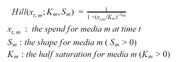
Equation 1. The Hill equation
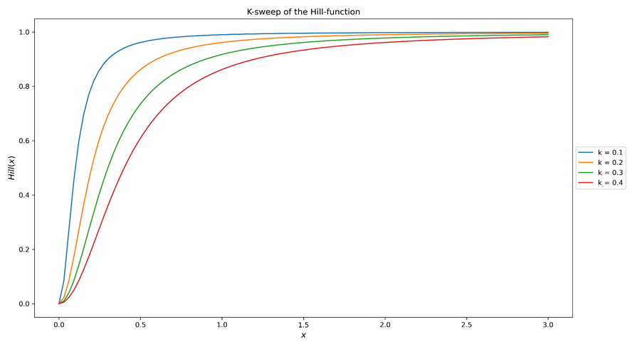
Figure 1a. Sweeping the K parameter (half-saturation) of the Hill function. The curve’s overall shape is roughly kept whilst the point of half saturation (where Hill(x)=0.5) is shifted. In other words, the bigger K is, the harder it is to saturate the associated media channel.
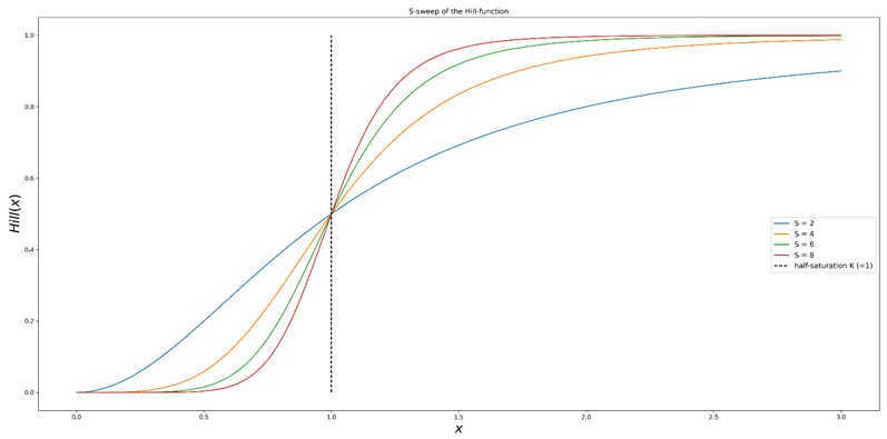
Figure 1b. Sweeping the S parameter (shape) of the Hill function. The curve’s half-saturation point is kept whilst the slope around it increases. In other words, the bigger S is, the bigger are the marginal gains for investments around the half saturation point.
As evidenced above, the Hill equation bears two important parameters: whilst K defines the point of half-saturation (the channel is at exactly half of its maximal revenue when investment equals K), S interferes with the shape of the saturation curve (the higher its value, the more S-shaped the curve becomes). Learning accurate estimations for K and S is essential because an optimal investment level can be analytically extracted from these parameters. Indeed, when no other effect is considered, the investment that yields maximum Return over Investment (ROI) can be calculated as:
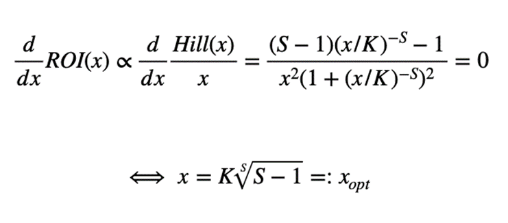
Equation 2. Deriving the optimal investment level from saturation parameters
Note that this optimal investment exists for S>1 and that it is always between one and three times the half-saturation value K (you can check this by verifying the values that the S-root can assume).
Time-delay
The second effect that should be considered is the revenue’s time allocation, after some channel-specific investment is executed. Indeed, investment and revenue do not occur simultaneously, and it might take a few weeks before the latter becomes significant. Furthermore, some media channels are bound to have more localized effects, whereas other channels can hold investments for longer periods of time, thus generating revenue even after relatively long periods of time. Both these aspects can be modeled via the Adstock equation given below, by the theta and alpha parameters respectively. The L parameter does not need to be specific to each channel and can only be set to a fixed value that is empirically known to be sufficiently large, such as L=13 (as suggested in [1]). Once again, the reader is invited to focus on Figures 2a and 2b instead of Equation 3.
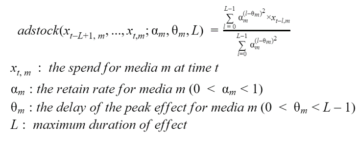
Equation 3. The Adstock equation
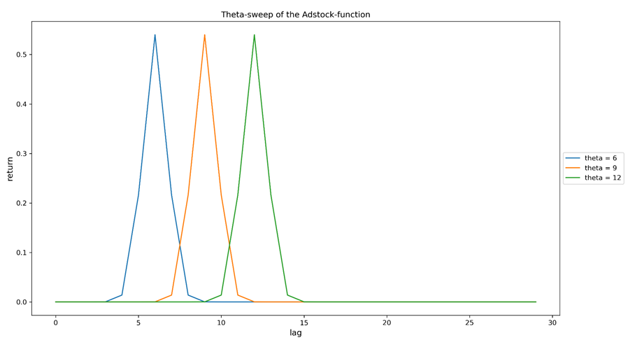
Figure 2a. Sweeping the theta parameter (peak delay) of the Adstock function. All curves are the result of a single investment made on lag=0 (lag can indicate whatever time granularity that was chosen in modelling). The larger theta is, the more time it takes for the maximal revenue to be observed, with relation to the investment that caused it.
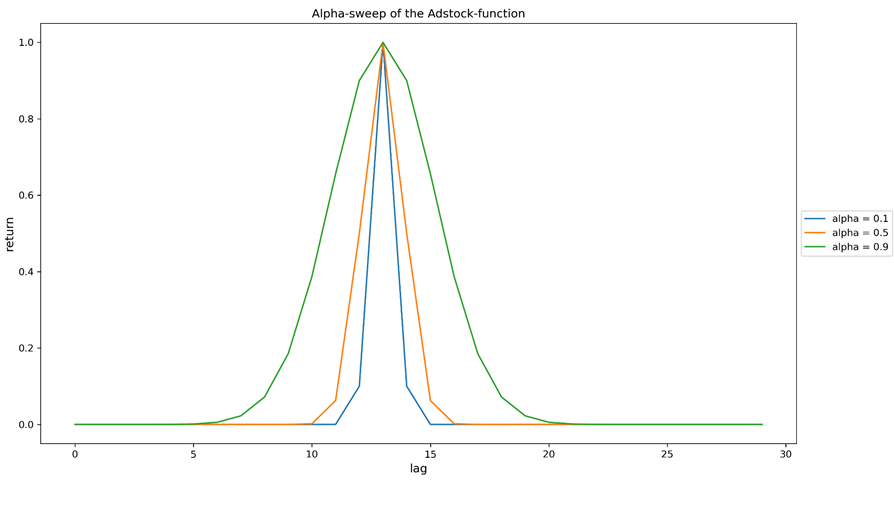
Figure 2b. Sweeping the alpha parameter (retain rate) of the Adstock function. All curves are the result of a single investment made on lag=0 (lag can indicate whatever time granularity that was chosen in modelling). The larger alpha is, the more delocalized is the revenue distribution. The curves were rescaled for better comparison.
Putting it all together: the Media Mix Modeling regression
Once both nonlinear mappings and their respective parameters are defined, the complete model can be given as follows:
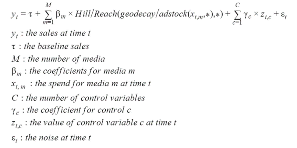
Equation 4. Media Mix Modeling regression equation
>Let’s start our analysis by breaking down the expression above. The first important observation is that all features are clustered into marketing investments and external (control) variables, with the most relevant difference being that the Hill and Adstock transformations are applied exclusively to the former. Note, thus, that the impact of control features is considered to be purely linear and immediate — even though trend and seasonality effects can be added through lag and seasonality features, respectively. Control variables can also be regarded as the set of factors outside of Marketing that have an impact on sales, including pricing, competitor sales etc. Other than the regression terms, we also account for a linear coefficient tau and a noise term epsilon.
>When all is included, this formulation engenders 4 nonlinear parameters for each marketing feature. Depending on the MMM’s scope and on how specifically all Marketing actions are regarded, our model may require several different marketing features, which makes the number of nonlinear parameters quite important. The way that these are treated in modeling implies different possible strategies, as will be discussed in what follows.
Why/When to go Bayesian?
The most perceptive readers might have noticed that Bayesian statistics were not even once evoked in the past sections. This begs the question: why should we care about using a Bayesian approach for fitting this model, when some specific observation data is available?
It turns out that the answer is very much related to the large number of parameters that must be approximated — a number which is quite often left unmatched by the data availability to fit our model. Let’s take a look at the Expertise x Data Availability matrix below:
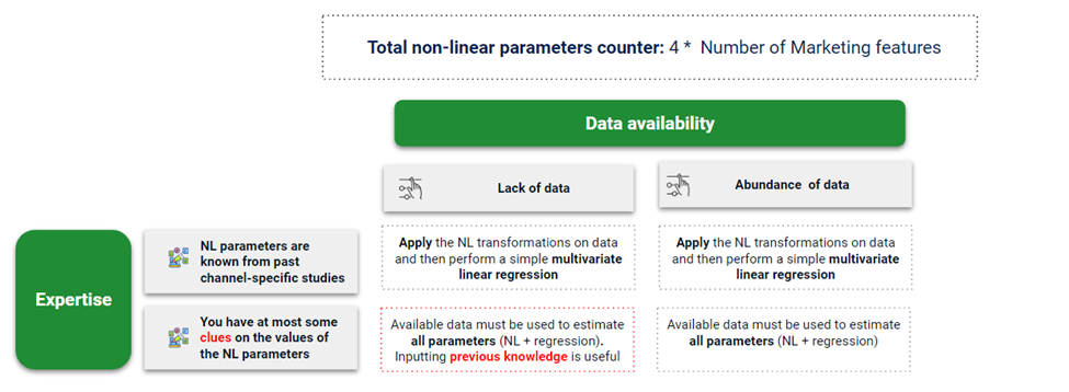
Figure 4.Expertise x Data Availability matrix for the Media Mix Modeling study
From this matrix, it should be clear that the complexity of the problem to be tackled here depends on the following question: is approximating all these nonlinear parameters part of our task? If not — that is, if these parameters are previously known — then they should only appear as pre-transformations to the data, which will then be fit into a simple linear multivariate regression model. This is ideally the case if enough past information/expertise is available to set approximate values to these parameters, and these values are simply not up to validation by data.
Needless to say, the absolute knowledge of channel behavior amongst all media types is quite a strong assumption, and chances are that at most some clues regarding these parameters are available for modeling. Hence, the observation data must also be used to fit these parameters and better understand the involved channels. If this is paired with low data availability, it becomes extremely convenient — or even required — to use all previously known information in order to guarantee good model performance.
The Bayesian approach is, thus, a way to perform an all-in-one estimation of parameters (regression and nonlinear), which allows for inputting clues to the model as prior knowledge, for best performance with limited data. Let’s now get a bit more into the details on how this can be achieved.
How to go Bayesian?
The Bayesian MMM adapts a set of prior distributions (one for the value of each linear or nonlinear parameter) into a set of posterior distributions. This is done by the exposure to data (evidence), and the posterior distributions can be regarded as revised understandings of how each channel behaves and contributes to sales. In Python, this can be implemented with probabilistic modeling libraries such as PySTAN or PyMC3.
Note that this strategy opens up a new set of controllable inputs, other than observation data: the prior distributions. Indeed, there is a lot of flexibility in the choice of distribution for every parameter and in tailoring their moments according to each channel, which will then result in a different output for the same observation data. Whereas the original Google article [1] reports distributions that were empirically observed to perform better for each parameter type (K, S, alpha, theta and beta), here we will explore how we can further tailor these to each individual channel according to previous knowledge on their behavior.
Less can be better
Before delving into prior distributions for each parameter, a potentially useful strategy to keep in mind is to verify if we cannot discard some of these parameters altogether. This will not only help us simplify the model but also (as a result) obtain a better performance in limited data.
Indeed, even though the nonlinear mappings are shown to be applied to all Marketing features in Equation 4, It might also be sensible to discard one or both transformations for some specific actions: for instance, if these features are extended to trade actions and not just media channels, one might be interested in including TPR (Temporary Price Reduction) investments as a feature. This has an obvious immediate effect, as sales lift is observed and killed off at virtually the same moment as the investment (price reduction) starts and seizes, respectively. Thus, there might be no interest in using the Adstock transformation for this feature, which has the benefit of reducing the number of parameters to be estimated.
Another viable simplification can be implemented for channels whose investments are known to vary very little in time: in these cases, we are operating at only a very small section of the curves shown in Figure 1, where the relation between return and investment can be deemed approximately linear. Hence, we can discard the Hill function for these channels, as saturation will not play an important role. In more technical terms, this assumption is valid when dx<<K, where dx is some measure of historical variation on investment.
Setting up a prior arsenal
Once the relevance of all nonlinear parameters is verified, the next step is to understand how their priors can bear information. So far, I have purposely used the rather technically vague term “clues” to define any kind of model input that is not structured, table-like observation data. Here we will take a look into some examples on what these could be and also fill the gap between these and the actual prior distributions that will serve as input for the Bayesian inference, carrying this knowledge into the model.
Let’s first take the example of price with relation to the competition. This is an external variable that inherently has a strong impact on sales, and could thus be included as a control feature in the MMM model. One could quite easily argue that the higher this relative price is, the lower the sales are going to be. This is common sense to us, but we should explicitly tell the model to only look for solutions with negative impact. The way that we do this is by choosing the prior distribution for the parameter beta associated to price (see Equation 4) to be a negative half normal. We do the opposite for positive-impact features (e.g. if you are modeling some refreshing beverage sales, the weekly average temperature should have a positive impact). Note that this is not a necessity: if you are not quite sure of a feature’s impact on the target variable, you can feed it an uninformed prior (e.g. the standard normal distribution) and let the model learn it by itself.
This is just an example of how to tune prior distributions in order to include qualitative knowledge in the model. Some other possible qualitative information can come from , for instance, a specific marketing action nature (as in the previously given example for TPR, if one decided to not cut the time-delay altogether but rather shift its distribution to concentrate on very short delays only). Quantitative prior knowledge, on the other hand, may come from previous studies or estimates performed on historical data analysis. As an example for the former, the regression weight distribution can be shifted according to the ROI value that was found in a previous MMM study — the model can then look for smaller/higher values from the start, for channels which are known to have smaller/bigger returns; as for the latter, the assumption that historical investments should be at roughly the same order as the ideal investment level can lead to informed priors on the saturation parameter K from Equation 1 — the model is, thus, informed of which channels are bigger or smaller in terms of potential reach.
The matrix below summarizes some key strategies that can be considered for tuning prior distributions, both qualitative and quantitative. This is not, by any means, an exhaustive list, and the viability of each may vary depending on the context and should be revised for each specific study.
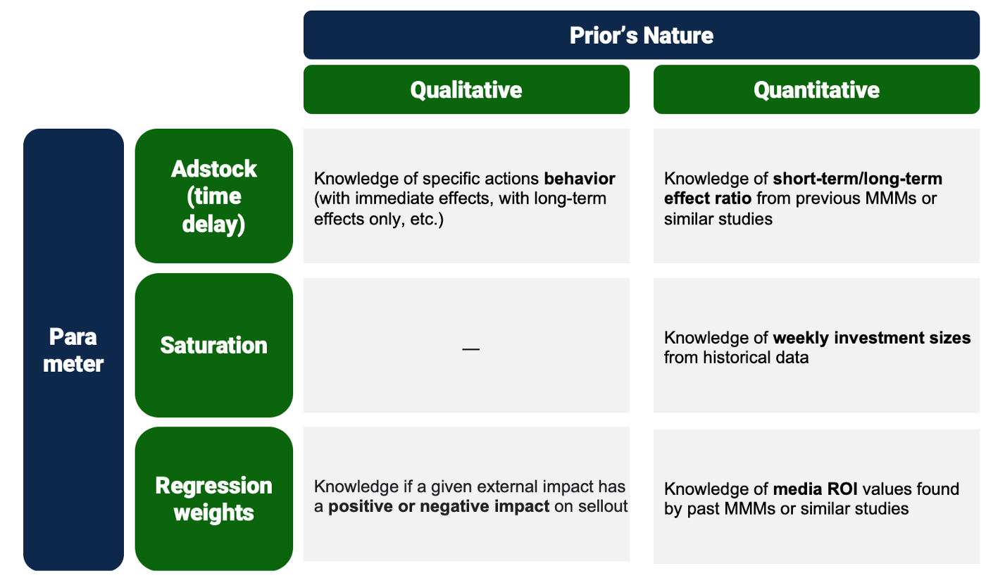
Figure 5. Example of a prior tuning strategy matrix for a use-case of the Bayesian Media Mix Modeling. Strategies should vary according to scope and available current knowledge
Conclusion and Take-home
Whereas an Media Mix Modeling study requires dealing with the behavior of several different Marketing actions, the Bayesian approach allows for an all-in-one estimation of these, alongside the sales lift for each one of these features as well as for external factors (control features). This allows us to harvest the available observed data in order to learn these behaviors when they are not known beforehand through some available expertise or past channel-specific studies and tests. Nevertheless, this comes with a cost, mostly reflected on the model’s complexity and the subsequent need of sufficient data to achieve a good performance. When this need is not met, a key result is a model which can quite easily overfit the observed data by giving out parameters that are simply not reasonable.
In this article, we have explored a way to remedy this effect by working with previous knowledge other than observable data, from quantitative conclusions in past studies to qualitative business understanding of some feature’s nature and impact on sales. These are included by tailoring the prior distributions of each one of the model’s parameters. Whereas in a pragmatic point of view this can be understood as biasing the model, it is also a way to avoid overfitting the model to patterns that are only observed due to the data’s limited availability, by focusing on combinations that are close to what is known or at least expected to be true. In other words, tailoring distributions is a way of compromising between learning from new observation data and respecting old business knowledge — a compromise that can be explored in several different levels according to what is available in a specific Media Mix Modeling case.
Acknowledgements
Special thanks to Camila C. Moreno, Rafael Melo, Rhayssa Sonohata, Vinicius Pacheco and Wedeueis Braz from the Brazilian Artefact team for reviewing this article before publication.

 BLOG
BLOG


