


Autor

Eine Schritt-für-Schritt-Anleitung zur Erfassung und Vorverarbeitung von Satellitenbildern data für Algorithmen des maschinellen Lernens
Dieser Artikel ist der erste Teil einer 2-teiligen Serie, die sich mit dem Einsatz von Algorithmen des maschinellen Lernens bei Satellitenbildern befasst. Hier konzentrieren wir uns auf die Schritte der data-Erfassung und -Vorverarbeitung, während im zweiten Teil die Verwendung verschiedener Algorithmen für maschinelles Lernen vorgestellt wird.
TL;DR
Dieser Artikel wird:
Wir werden die Erkennung und Klassifizierung von landwirtschaftlichen Feldern als Beispiel verwenden. Für die Vorverarbeitungsschritte werden Python und Jupyter Notebook verwendet. Das Jupyter-Notebook zum Nachvollziehen der Schritte ist auf Github verfügbar.
Dieser Artikel setzt grundlegende Kenntnisse in data Wissenschaft und Python voraus.
Computer Vision ist ein faszinierender Zweig des maschinellen Lernens, der sich in den letzten Jahren schnell entwickelt hat. Mit dem öffentlichen Zugang zu vielen Algorithmenbibliotheken von der Stange (Tensorflow, OpenCv, Pytorch, Fastai ...) sowie die quelloffenen data-Sets (CIFAR -10, Imagenet, IMDB ...) ist es für einen data-Wissenschaftler sehr einfach, praktische Erfahrungen zu diesem Thema zu sammeln.
Aber wussten Sie, dass Sie auch auf Open-Source-Satellitenbilder zugreifen können? Diese Art von Bildmaterial kann in einer Vielzahl von Anwendungsfällen (Landwirtschaft, Logistik, Energie ...) verwendet werden. Allerdings stellen sie aufgrund ihrer Größe und Komplexität zusätzliche Herausforderungen für einen data-Wissenschaftler dar. Ich habe diesen Artikel geschrieben, um einige meiner wichtigsten Erkenntnisse aus der Arbeit mit diesen Bildern mitzuteilen.
Schritt 1 - Wählen Sie die Quelle Satellite open data
Zunächst müssen Sie den Satelliten auswählen, den Sie verwenden möchten. Die wichtigsten Merkmale, auf die Sie achten sollten, sind:
Hier sind die Satelliten, deren data kostenlos verfügbar sind:
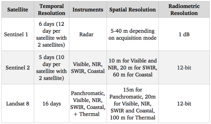
Benchmark der Satellitensysteme
Da unser Ziel darin besteht, landwirtschaftliche Nutzpflanzen zu erkennen und zu identifizieren, sollte das sichtbare Spektrum (das zur Erstellung von Standardfarbbildern verwendet wird) recht nützlich sein. Außerdem gibt es Korrelationen zwischen dem Stickstoffgehalt von Pflanzen und den NIR-Spektralbändern (Nahinfrarot). Was die kostenlosen Optionen angeht, so ist Sentinel 2 mit 10 m für diese Spektralbänder derzeit die beste Auflösung, also werden wir diesen Satelliten verwenden.
Natürlich ist die Auflösung von 10 m im Vergleich zum aktuellen Stand der Technik bei Satellitenbildern viel geringer, da kommerzielle Satelliten eine Auflösung von 30 cm erreichen. Der Zugang zu kommerziellen data-Satelliten kann viele Anwendungsfälle erschließen, aber trotz des zunehmenden Wettbewerbs durch neue Anbieter, die in diesen Markt eintreten, sind sie nach wie vor hochpreisig und daher schwer in einen skalierten Anwendungsfall zu integrieren.
Schritt 2 - Sammeln Sie die Satellitenbilder data von Sentinel 2
Nachdem wir nun unsere Satellitenquelle ausgewählt haben, besteht der nächste Schritt darin, die Bilder herunterzuladen. Sentinel 2 ist Teil des Copernicus-Programms der Europäische Weltraumorganisation. Wir können auf seine data über den Befehl SentinelSat python API.
Zunächst müssen wir ein Konto bei der Copernicus Open Access Hub. Alternativ können Sie auf dieser Website auch Bilder mit einer grafischen Benutzeroberfläche abfragen.
Sie können die Zonen, die Sie erkunden möchten, angeben, indem Sie der API eine Geojson-Datei zur Verfügung stellen. Dabei handelt es sich um eine json-Datei, die die GPS-Koordinaten (Breiten- und Längengrad) einer Zone enthält. Geojson kann schnell erstellt werden auf dieser Website.
Auf diese Weise können Sie alle Satellitenbilder abfragen, die sich mit der angegebenen Zone überschneiden.
Hier listen wir alle Bilder auf, die für eine bestimmte Zone und einen bestimmten Zeitraum verfügbar sind:
api = SentinelAPI(
credentials[“username”],
credentials[“Passwort”],
“https://scihub.copernicus.eu/dhus”
)
shape = geojson_to_wkt(read_geojson(geojson_path))
images = api.query(
Form,
date=(date(2020, 5, 1), date(2020, 5, 10)),
platformname=”Sentinel-2″,
Verarbeitungsstufe = “Level-2A”,
cloudDeckungsprozentsatz=(0, 30)
)
images_df = api.to_dataframe(images)
Beachten Sie die Verwendung von Argumenten:
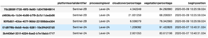
bilder_df
Images_df ist ein Pandas dataframe, das alle Bilder enthält, die unserer Abfrage entsprechen. Wir wählen eines mit einer niedrigen cloud-Abdeckung aus und laden es mit der api herunter:
api.download(uuid)
Schritt 3 - Verstehen Sie, welche Spektralbänder verwendet werden sollen und verwalten Sie die Quantisierung
Sobald die Zip-Datei heruntergeladen ist, können wir sehen, dass sie tatsächlich mehrere Bilder enthält.
Das liegt daran, dass Sentinel 2, wie bereits in Schritt 1 erwähnt, viele Spektralbänder und nicht nur Rot, Grün und Blau aufnimmt und jedes Band in einem einzigen Bild erfasst wird.
Auch die Instrumente haben nicht alle die gleiche räumliche Auflösung, daher gibt es einen Unterordner für die verschiedenen Auflösungen 10, 20 und 60 Meter.
Wenn wir die GRANULE//IMG_DATA sehen wir, dass es für jede unterschiedliche Auflösung einen Unterordner gibt: 10, 20 und 60 Meter als die Spektralbänder. Wir werden die Bänder mit der maximalen Auflösung 10 m verwenden, da sie die Bänder 2, 3, 4 und 8 enthalten, die Blau, Grün, Rot und NIR sind. Die Bänder 7, 8 und 9, bei denen es sich um den roten Rand der Vegetation handelt (Spektralbänder zwischen Rot und NIR, die einen Übergang im Reflexionswert der Vegetation markieren), könnten ebenfalls für die Erkennung von Pflanzen interessant sein, aber da sie eine geringere Auflösung haben, lassen wir sie jetzt beiseite
Hier laden wir jedes Band als 2D-Numpy-Matrix:
def get_band(bild_ordner, band, auflösung=10):
subfolder = [f for f in os.listdir(image_folder + "/GRANULE") if f[0] == "L"][0]
bild_ordner_pfad = f"/GRANULE//IMG_DATA/Rm"
image_files = [im for im in os.listdir(image_folder_path) if im[-4:] == ".jp2"]
selected_file = [im for im in image_files if im.split("_")[2] == band][0]
with rasterio.open(f"/") as infile:
img = infile.read(1)
return img
band_dict =
für Band in ["B02", "B03", "B04", "B08"]:
band_dict[band] = get_band(bild_ordner, band, 10)
Ein schneller Test, um sicherzustellen, dass alles funktioniert, ist der Versuch, das Bild in Echtfarbe (d.h. RGB) zu erstellen und es mit opencv und matplotlib anzuzeigen:
img = cv2.merge((band_dict[“B04”], band_dict[“B03”], band_dict[“B02”]))
plt.imshow(img)
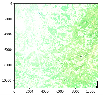
Satellitenbild - Problem mit der Farbintensität (Copernicus Sentinel data 2020)
Allerdings gibt es ein Problem mit der Farbintensität. Das liegt daran, dass die Quantisierung (Anzahl der möglichen Werte) vom Standard für Matplotlib abweicht, der entweder einen 0-255 int-Wert oder einen 0-1 float-Wert annimmt. Standardbilder verwenden oft eine 8-Bit-Quantisierung (256 mögliche Werte), aber Sentinel 2-Bilder verwenden eine 12-Bit-Quantisierung und eine Nachbearbeitung konvertiert die Werte in eine 16-Bit-Ganzzahl (65536 Werte).
Wenn wir eine 16-Bit-Ganzzahl auf eine 8-Bit-Ganzzahl skalieren wollen, sollten wir theoretisch durch 256 teilen, aber das führt zu einem sehr dunklen Bild, da nicht der gesamte Bereich der möglichen Werte genutzt wird. Der Maximalwert in unserem Bild ist 16752 von 65536 und nur wenige Pixel erreichen Werte über 4000, so dass die Teilung durch 8 tatsächlich ein Bild mit einem ordentlichen Kontrast ergibt.
img_processed = img / 8
img_processed = img_processed.astype(int)
plt.imshow(img_processed)
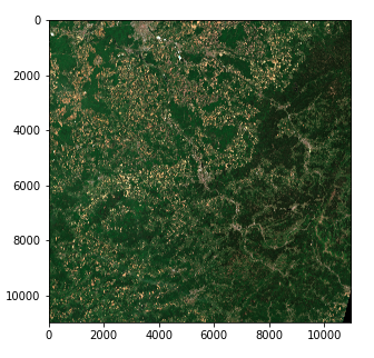
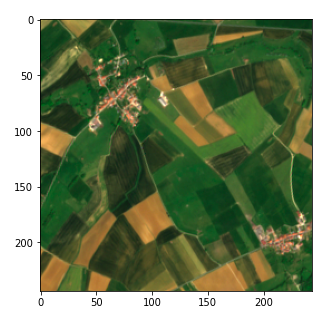
Satellitenbild - Rechte Farbintensität (Copernicus Sentinel data 2020)
Wir haben nun einen 3-dimensionalen Tensor der Form (10980, 10980, 3) aus 8-Bit-Ganzzahlen in Form eines Numpy-Arrays
Beachten Sie, dass :
Schritt 4 - Teilen Sie die Bilder in für das maschinelle Lernen geeignete Größen auf.
Wir könnten versuchen, einen Algorithmus auf unser aktuelles Bild anzuwenden, aber in der Praxis würde das mit den meisten Techniken aufgrund der Größe des Bildes nicht funktionieren. Selbst mit starker Rechenleistung wären die meisten Algorithmen (und insbesondere Deep Learning) vom Tisch.
Wir müssen das Bild also in Fragmente aufteilen. Eine Frage ist, wie wir die Größe der Fragmente festlegen.
Wir entscheiden uns dafür, jedes Bild in ein 45 * 45 Raster aufzuteilen (45 ist praktischerweise ein Teiler von 10980)
Nach der Festlegung der Parameter ist dieser Schritt mit Hilfe der Numpy-Array-Manipulation ganz einfach. Wir speichern unsere Werte in einem dict mit (x, y) Tupeln als Schlüssel.
frag_count = 45
frag_size = int(img_processed.shape[0] / frag_count)
frag_dict =
for y, x in itertools.product(range(frag_count), range(frag_count)):
frag_dict[(x, y)] = img_processed[y*frag_size: (y+1)*frag_size,
x*frag_size: (x+1)*frag_size, :]
plt.imshow(frag_dict[(10, 10)])
Fragment des Satellitenbildes (Copernicus Sentinel data 2020)
Schritt 5 - Verknüpfen Sie Ihr data mit den Satellitenbildern, indem Sie GPS in UTM konvertieren
Schließlich müssen wir unsere Bilder mit den data, die wir über landwirtschaftliche Felder haben, verknüpfen, um einen überwachten maschinellen Lernansatz zu ermöglichen. In unserem Fall haben wir data auf landwirtschaftlichen Feldern in Form einer Liste von GPS-Koordinaten (Breitengrad, Längengrad), ähnlich dem Geojson, das wir in Schritt 2 verwendet haben, und wir möchten in der Lage sein, ihre Pixelposition zu finden. Der Übersichtlichkeit halber zeige ich Ihnen zunächst die Konvertierung von Pixeln in GPS-Koordinaten und dann die Umkehrung
Die metadata, die bei der Abfrage der SentinelSat-API erfasst wurde, liefert die GPS-Koordinaten der Ecken des Bildes (Footprint-Spalte) und wir möchten die Koordinaten eines bestimmten Pixels. Die Längen- und Breitengrade, bei denen es sich um Winkelwerte handelt, entwickeln sich innerhalb eines Bildes nicht linear, so dass wir kein einfaches Verhältnis anhand der Pixelposition erstellen können. Es gibt Möglichkeiten, dieses Problem mit mathematischen Gleichungen zu lösen, aber es gibt bereits fertige Lösungen in Python.
Eine schnelle Lösung besteht darin, die Pixelposition in UTM (Universal Transverse Mercator) zu konvertieren, bei dem eine Position durch eine Zone sowie eine (x, y) Position (in der Einheit Meter) definiert ist, die sich linear mit dem Bild entwickelt. Wir können dann eine Konvertierung von UTM in Latitude / Longitude verwenden, die in der utm-Bibliothek zur Verfügung steht. Dazu müssen wir zunächst die UTM-Zone und die Position der linken oberen Ecke des Bildes ermitteln, die Sie in metadata des Echtfarbbildes finden.
#Oerhält meatadata
transform = rasterio.open(tci_file_path, driver=’JP2OpenJPEG’).transform
zone_number = int(tci_file_path.split(“/”)[-1][1:3])
zone_letter = tci_file_path.split(“/”)[-1][0]
utm_x, utm_y = transform[2], transform[5]
# Konvertierung der Pixelposition in utm
east = utm_x + pixel_column * 10
Norden = utm_y + pixel_row * - 10
# Konvertierung von UTM in Breiten- und Längengrad
Breitengrad, Längengrad = utm.to_latlon(east, north, zone_number, zone_letter)
Die Umwandlung der GPS-Position in Pixel erfolgt mit den umgekehrten Formeln. In diesem Fall müssen wir sicherstellen, dass die erhaltene Zone mit unserem Bild übereinstimmt. Dies können Sie tun, indem Sie die Zone angeben. Wenn unser Objekt nicht im Bild vorhanden ist, führt dies zu einem unzulässigen Pixelwert.
# Konvertierung von Breiten- und Längengraden in UTM
east, north, zone_number, zone_letter = utm.from_latlon(
Breitengrad, Längengrad, force_zone_number=zone_number
)
# Konvertierung von UTM in Spalte und Zeile
pixe_column = round((east - utm_x) / 10)
pixel_row = round((nord - utm_y) / -10)
roh ansehen
Fazit
Wir sind nun bereit, die Satellitenbilder für das maschinelle Lernen zu verwenden!
Im nächsten Artikel dieser 2-teiligen Serie werden wir sehen, wie wir diese Bilder verwenden können, um Feldoberflächen mithilfe von überwachtem und unüberwachtem maschinellen Lernen zu erkennen und zu klassifizieren.
Danke fürs Lesen und zögern Sie nicht Folgen Sie dem Artefact Technik-Blog wenn Sie benachrichtigt werden möchten, wenn der nächste Artikel erscheint!