

Auteur


La modélisation de la propension peut être utilisée pour augmenter l'impact de votre communication avec les clients et optimiser vos dépenses publicitaires.
Google Analytics data est une source data bien structurée qui peut facilement être transformée en un ensemble data prêt pour l'apprentissage automatique.
Les tests rétrospectifs sur l'historique de data et les mesures techniques peuvent vous donner une première idée de la performance de votre modèle, tandis que les tests en direct et les mesures commerciales vous permettront de confirmer l'impact de votre modèle.
Notre modèle d'apprentissage automatique personnalisé a surpassé les références existantes : lors des tests en direct en termes de ROAS (retour sur investissement publicitaire) : +221% par rapport au modèle basé sur des règles et +73% par rapport au modèle d'apprentissage automatique standard (score de qualité des sessions Google Analytics).
Cet article part du principe que les bases de l'apprentissage automatique et du marketing sont fondamentales.
Qu'est-ce que la modélisation de la propension ?
La modélisation de la propension est estimer la probabilité qu'un client effectue une action donnée. Plusieurs actions peuvent être utiles à l'estimation :
Dans cet article, nous nous concentrerons sur l'estimation de la propension à acheter un article sur un site web de commerce électronique.
Mais pourquoi estimer la propension à l'achat ? Parce qu'elle permet deadapter la façon dont nous voulons interagir avec un client. Supposons, par exemple, que nous disposions d'un modèle de propension très simple qui classe les clients en “froids”, “tièdes” et “chauds” pour un produit donné (“chauds” étant les clients qui ont le plus de chances d'acheter et “froids” ceux qui en ont le moins) :
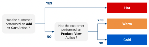
Sur la base de cette classificationvous pouvez avoir une réponse ciblée spécifique pour chaque classe. Vous pourriez vouloir adopter une approche marketing différente selon qu'il s'agit d'un client très proche de l'achat ou d'un client qui n'a peut-être même jamais entendu parler de votre produit. De même, si vous disposez d'un budget média limité, vous pouvez le concentrer sur les clients qui ont une forte probabilité d'acheter et ne pas trop dépenser pour ceux qui ont peu de chances d'acheter.
Ce type simple de classification basée sur des règles peut donner de bons résultats et est généralement préférable à l'absence de classification, mais il présente les inconvénients suivants plusieurs limites :
Pour faire face à ces limitations, nous pouvons utiliser une approche plus orientée data : utilisez apprentissage automatique sur notre data pour prévoir une probabilité d'achat pour chaque client.
Comprendre Google Analytics data
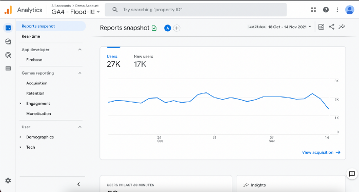
Google Analytics est un outil service web d'analyse qui suit l'utilisation data et le trafic sur le site web et les applications.
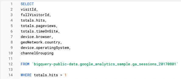
Google Analytics data peut être facilement exporté vers Big Query (Google Cloud Platform entièrement géré data service entrepôt) où il est possible d'y accéder via une syntaxe de type SQL :
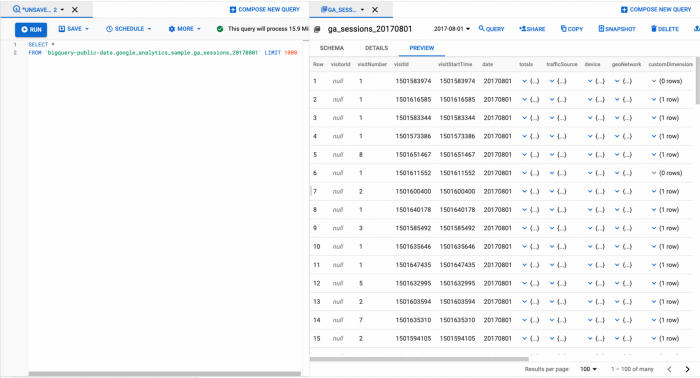
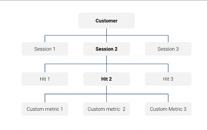
Notez que le tableau d'exportation Big Query avec Google Analytics data est un tableau d'exportation de données. tableau imbriqué au niveau de la session :
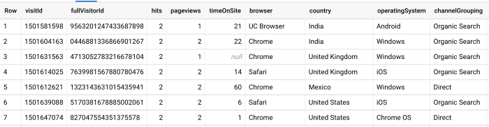
Par exemple, dans cette requête, nous recherchons uniquement caractéristiques au niveau de la session:
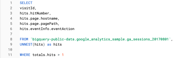
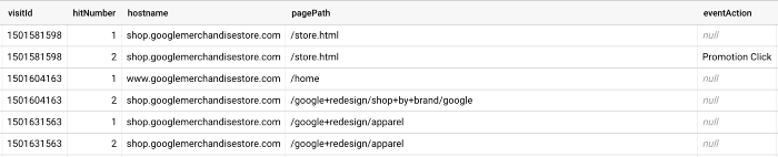
Dans cette requête, nous avons utilisé une fonction Unnest pour obtenir les mêmes informations à l'adresse suivante niveau d'atteinte:
Pour plus d'informations sur le GA data, consultez la page documentation. Notez que notre projet a été développé sur GA360, donc si vous utilisez la dernière version, GA4, il y aura de légères différences dans le modèle data, en particulier le tableau sera au niveau de l'événement. Il existe des tableaux d'exemples publics de GA360 et GA4 data disponible sur Big Query.
Maintenant que nous avons accès à notre source brute data, nous devons procéder à l'ingénierie des caractéristiques avant d'introduire notre tableau dans un algorithme d'apprentissage automatique.
Concevoir les bonnes caractéristiques
L'objectif de l'étape d'ingénierie des caractéristiques est de transformer les données brutes de Google Analytics data (extraites de Big Query) en une base de données d'analyse des caractéristiques. table prête à utiliser pourApprentissage automatique.
GA data est très bien structuré et ne nécessitera qu'un minimum d'étapes de nettoyage. Cependant, le tableau contient encore de nombreuses informations, dont beaucoup ne sont pas utiles pour l'apprentissage automatique ou ne peuvent pas être utilisées telles quelles, c'est pourquoi il est important de sélectionner et d'élaborer les bonnes caractéristiques. C'est pourquoi il est important de sélectionner et d'élaborer les bonnes caractéristiques. Pour ce faire, nous avons construit des caractéristiques qui semblaient être les plus corrélées à l'achat d'un produit.
Nous avons élaboré 4 types de caractéristiques :
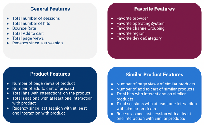
Notez que nous calculons toutes ces caractéristiques au niveau du client, ce qui signifie que nous agrégeons des informations provenant de plusieurs sessions pour chaque client (en utilisant le champ fullVisitorId comme clé).
Caractéristiques générales
Les caractéristiques globales sont les suivantes caractéristiques numériques qui donnent des informations générales sur la session.
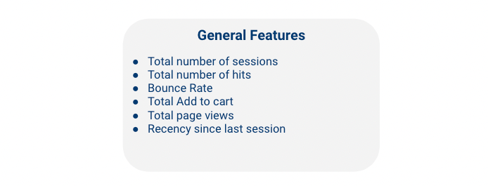
Notez que le taux de rebond est défini comme % de fois où le client n'a visité qu'une seule page web au cours d'une session.
Il était également important d'inclure des informations sur les la récurrence des événementsLe site web de l'entreprise est un outil de gestion de la relation client : par exemple, un client qui vient de visiter votre site web est probablement plus enclin à acheter qu'un client qui l'a visité il y a trois mois. Pour plus d'informations sur ce sujet, vous pouvez consulter la théorie sur le site suivant RFM (récence, fréquence, valeur monétaire).
Nous avons donc ajouté une fonctionnalité Récence depuis la dernière session = 1 / Nombre de jours depuis la dernière session qui permet de normaliser la valeur entre 0 et 1
Caractéristiques préférées
Nous avons également voulu inclure des informations sur la clé catégorielle data disponibles, tels que navigateur ou appareil. Étant donné que ces informations se situent au niveau de la session, il peut y avoir plusieurs valeurs différentes pour un même client. Nous ne retenons donc que celle qui apparaît le plus souvent par client (c'est-à-dire la préférée). De même, pour éviter d'avoir des caractéristiques catégorielles avec une cardinalité trop élevée, nous ne conservons que les 5 valeurs les plus courantes pour chaque caractéristique et remplaçons toutes les autres valeurs par une valeur “Autre”.

Caractéristiques du produit
Si les deux premiers types de caractéristiques sont certainement utiles pour répondre à la question “Un client va-t-il acheter sur mon site web ?”, ils ne sont pas suffisamment précis pour nous permettre de savoir “Le client va-t-il acheter un produit spécifique ?”. Pour répondre à cette question, nous avons créé des caractéristiques spécifiques au produit qui ne comprennent que le produit pour lequel nous essayons de prédire l'achat :
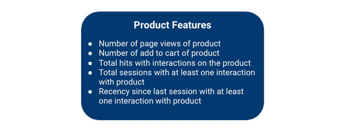
Pour Récence depuis la dernière session avec au moins une interaction avec ce produit, nous utilisons la même formule que pour le Récence de la session dans les caractéristiques générales. Cependant, il peut arriver qu'il n'y ait aucune session avec au moins une interaction avec le produit, auquel cas nous remplissons le champ avec 0. Cela est logique d'un point de vue commercial puisque la valeur la plus élevée possible est 1 (lorsque le client a eu une session depuis hier).
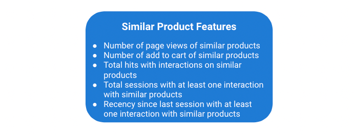
Caractéristiques similaires du produit
Outre l'interaction du client avec le produit pour lequel nous essayons de prédire la probabilité d'achat, le fait de savoir que le client a interagi avec d'autres produits ayant une fonction et un prix similaires peut certainement être utile (c'est-à-dire un produit de substitution). C'est pourquoi nous avons ajouté un ensemble de caractéristiques de produits similaires qui sont identiques aux caractéristiques de produits, sauf que nous incluons également les produits similaires dans la portée de la variable. Les produits similaires pour un produit donné ont été définis à l'aide de données commerciales.
Nous avons maintenant notre Caractéristiques de l'ensemble dataset sur lequel nous pouvons former notre modèle d'apprentissage automatique.
Formation du modèle
Puisque nous voulons savoir si un client va acheter un produit spécifique ou non, il s'agit d'une problème de classification binaire.
Pour notre première itération, nous avons procédé comme suit pour créer notre ensemble dataset d'apprentissage automatique (1 ligne par client) :
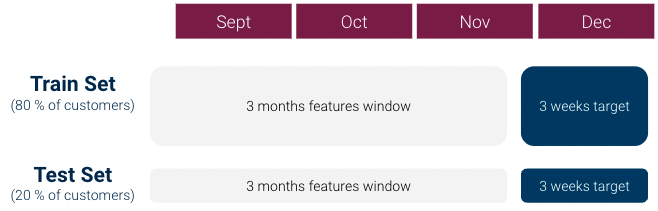
Cependant, une première exploration data a rapidement montré qu'il existait une problème de fort déséquilibre entre les classes: Le ratio classe 1 / classe 0 était supérieur à 1:1000 et nous n'avions pas assez de clients de classe 1. Cela peut être très problématique pour les modèles d'apprentissage automatique.
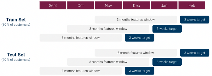
Pour faire face à ces problèmes, nous avons apporté plusieurs modifications à notre approche :
En utilisant ce dataset, nous avons testé plusieurs modèles de classification : Modèle linéaire, Random Forest et XGboost, en affinant les hyperparamètres à l'aide d'une grille de recherche, et nous avons fini par sélectionner un modèle de classification de type Modèle XGboost.
Évaluation de notre modèle
Lors de l'évaluation d'un modèle de propension, deux types principaux d'évaluations peuvent être effectués :
Évaluation du backtest
Tout d'abord, nous avons effectué évaluation du backtest: nous avons appliqué notre modèle à passé historique data et vérifié que notre modèle identifie correctement les clients qui vont effectuer un ajout au panier. Comme nous utilisons un classificateur binaire, le modèle produit un score de probabilité entre 0 et 1 d'être de la classe 1 (Ajouter au panier).
matrice de confusion et calculez la précision / rappel (ou leur forme combinée dans lescore f1). Ces mesures simples posent toutefois deux problèmes :
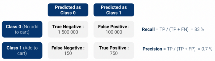
Nous avons donc décidé d'utiliser deux mesures qui étaient plus interprétable:
Les résultats de ces mesures ont été plutôt positifs, en particulier, Uplift était aux alentours de 13.5.
L'évaluation du backtest est une méthode sans risque pour une première évaluation d'un modèle de propension, mais elle présente plusieurs limites :
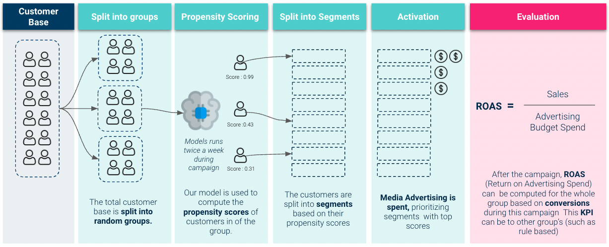
Évaluation du Livetest
Pour avoir une meilleure idée de la valeur commerciale de notre modèle, nous devons donc effectuer les opérations suivantes test d'évaluation en direct. Ici, nous activons notre modèle et l'utilisons pour hiérarchiser les dépenses de budget publicitaire :
Les résultats que nous avons obtenus lors du test en direct étaient très solides :
Pour conclure
En plus d'atteindre de bonnes performances, notre approche présente l'avantage d'être très générique. Presque aucune des étapes de l'ingénierie des caractéristiques ne doit être adaptée pour appliquer notre modèle à un un champ d'application national ou un champ d'application de produit différent. En fait, après notre premier succès dans le test en direct, nous avons pu déployer notre modèle dans plusieurs pays et pour plusieurs produits de manière très efficace.
Je vous remercie de votre lecture. Je serais heureux d'entendre vos commentaires sur cette approche. Avez-vous déjà construit des modèles de propension ? Si oui, qu'avez-vous fait différemment ?
Merci à Bruce Delattre, Rafaëlle Aygalenq et Cédric Ly.