

作者

更好地考虑促销 data 的 5 个技巧
简要说明
在这篇关于需求预测的大型系列文章中,我们将重点讨论如何为促销建模,促销是销售预测中的一个关键驱动因素,我们将研究典型的促销 dataset 是什么样的,应该如何制作特征,并用 Python 逐步举例说明,以及如何处理复杂的促销粒度。.
背景
作为零售商,在预测需求时,我们通常可以利用一些有用的 data 资料来源,如历史销量、产品和客户层次、节假日、售罄和促销活动。需要特别注意的是促销活动,因为在现实生活中,促销活动往往不仅仅是一个虚假的标志,你应该把它作为一个特征添加到你的模型中。它是一种真正复杂的商业机制,如果处理得当,可以为模型带来额外的性能。.
提示 1:了解促销参考信息
销售 dataset 通常不包括促销 data。您需要在培训 data 中插入特定的参考资料。促销 data 通常是一组列,以促销计划的格式出现,具有促销特征,例如:
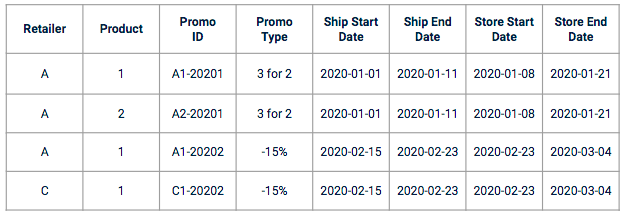
促销示例 data
在开始特征工程和建模部分之前,建议与业务所有者进行访谈,以了解如何创建和处理推广。让我们以日期为例。在卖出预测的情况下,促销会与多个日期相关联:
了解哪些日期对目标变量的影响最大,并与企业主确认是否有任何特殊情况需要考虑(例如,某些零售商可能会在正式开始和结束日期之前或之后实施促销活动),这一点非常重要。.
执行探索性 Data 分析 (EDA) 可以帮助您了解促销对目标变量的波动和影响。例如,从下图可以看出,某类促销活动比其他促销活动的影响更大。.
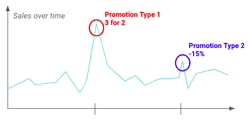
举例说明两种不同促销活动对特定产品销售的影响
EDA 还可用于验证业务团队之前强调的见解。下面,零售商似乎早在正式开始日期之前就开始了促销活动。.
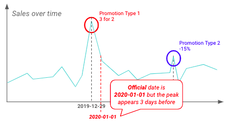
正式晋升日期与实际晋升日期之间的差异示例
在探索之后,我们需要对原始推广 data 进行处理,以便使用。首先要对日期进行扩展和处理,以便有一个连续的时间轴。其中一些日期可能需要根据探索和业务访谈阶段的发现进行调整。.
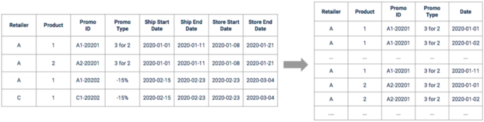
促销活动 data 在预处理前后的图示
提示 2:选择正确的粒度
正如您的 EDA 所显示的,促销对不同产品、零售商(或店铺,如果您使用的是售罄的 data)和促销类型的影响大不相同。理想情况下,您希望尽可能精确,并保持 SKU x 零售商 x 促销类型的粒度。.
例如,您可能有两种不同的地理粒度:零售商和仓库(即一个仓库包含多个零售商)。通过绘制每个粒度的时间序列图,您可能会发现促销的影响在零售商层面上非常明显,但在仓库层面上似乎被抹平了。这是因为并非仓库中的所有零售商都以同样的方式受到促销的影响。因此,在这个例子中,最好以零售商为粒度进行分析。.
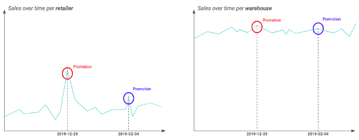
粒度不同,晋升影响也不同
一旦 EDA 完成,促销 data 的粒度正确,我们的目标就是为未来计划的促销活动创建最相关的特征,并预测相关的销售额。.
秘诀 3:设计正确的功能
人们可能会认为,只要在训练 dataset 中添加一个虚拟变量就足够了。这样做的目的是引导模型理解需求或销售额在某个时间点较高的原因。然而,这种方法并不能很好地模拟促销对销售的影响。通常情况下,某些促销类型可能比其他促销类型更有效,促销的影响也可能在开始日期附近更大,而在开始日期之后则较小(因为很少有人能从促销中获益)。.
在使用提升算法时,我们发现一个更复杂的功能非常有用,那就是计算销售额滚动平均值,以便让模型深入了解每种促销类型在过去的成功率有多高。.
1.理论
这种功能背后的理念是,针对给定的促销活动,衡量过去 “类似促销活动 ”最近产生的平均销量。我们将在一个给定范围的滚动窗口(如过去 7 天)上计算类似范围(相同促销类型、相同 SKU、相同零售商)的平均历史销售量。.
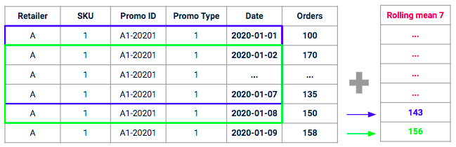
7 天窗口滚动平均值示例
对于这类功能,应特别注意 data 的泄漏,尤其是在设置时间跨度时。.
2.Python 实现
让我们看看如何在 Python 中逐步实现 7 天滚动平均值功能。首先,用以下信息定义我们的 DataFrame:
# 初始化我们的示例 dataframe,其中包含 6 列:SKU、零售商、促销类型、,
# 促销编号、日期、销售日期
df = pd.DataFrame(
)
# 初始化我们的视野:7 天滚动平均值
地平线 = 7
# 增加一行 "将来",我们希望对其卖出量进行预测(未知数为
#),因此我们希望为其提供一个滚动平均特征值
df = df.append(
,
ignore_index=True
)
创建完成后,我们的 DataFrame 看起来就像这样:
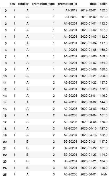
初始 DataFrame
接下来,我们将创建两个重要列:晋升开始日期和滚动平均值 (暂无).
# 我们创建两个新列:
# - 最短促销日期(根据促销 ID 确定的开始日期)
df = df.merge(
df.groupby(["sku", "retailer", "promotion_id"]).date.min()
.reset_index()
.rename(columns=)、,
on=["sku", "retailer", "promotion_id"]、,
how="left"
)
df = df.sort_values("min_promo_date")
# - 滚动平均值特征,暂时用 NaN 填充
df['promo_rolling_mean'] = np.nan
现在,DataFrame 应该是这样的:
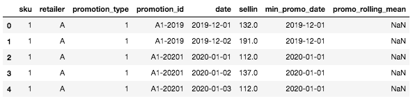
带有两个新立柱的 DataFrame 的头部
在此基础上,我们可以开始填写促销活动的平均值列。请记住,我们的目标是计算以往类似促销活动的平均售出量,但 相似性概念可能很棘手. .最好的情况是,在我们的历史记录中,同一零售商、同一 SKU 有相同类型的促销活动。最坏的情况是,有一个新的促销活动,其类型是新的,我们没有任何 SKU 和零售商的历史记录。因此,我们的想法是定义几个粒度级别,从最细粒度级别(如 SKU x 零售商 x 促销类型)到最 小粒度级别(如 SKU),查看是否有历史记录,从而计算滚动平均值。.
例如,SKU:1,零售商:A,促销类型:1,日期:2020-01-01。我们查找过去类似的促销活动。幸运的是,在 2019 年(promotion_id = ‘A1-2019’),针对相同的 SKU、相同的零售商(即最细粒度的级别),已经有一次促销活动采用了相同的促销类型。因此,我们将取最近 7 个发生此类促销的日期的销售量平均值。在其他情况下,我们可能找不到与这一粒度匹配的数据,因此我们只能通过 SKU 和促销类型来查找匹配数据。同样,如果没有匹配,我们最后将只取 SKU 级别的平均值。.
# 确定计算滚动平均值的粒度等级,从最细粒度开始
# 到粒度较小的
AGG_LEVELS =
# 我们会在以下表格中遍历粒度级别(从粒度最高的到粒度较低的
# 以计算每行最相似促销活动的滚动平均值
对于 AGG_LEVELS.items()中的 agg_level_number、agg_level_columns:
# 一旦滚动平均值特征被填满,我们就会脱离循环
if df["promo_rolling_mean"].isna().sum() == 0:
断裂
# (1) 我们将 data 框架汇总到当前粒度级别
agg_level_df = df.groupby(["promotion_id"] + agg_level_columns)
.agg()
.reset_index()
.rename(columns=)
.dropna(subset=["sellin"])
.sort_values("min_promo_date")
# (2) 我们计算当前粒度在给定范围内的滚动平均值
# 级
agg_level_df["sellin"] = agg_level_df.groupby(agg_level_columns)
.rolling(horizon, 1)["sellin"].
.mean()
.droplevel(
level=list(
range(len(agg_level_columns))
)
)
# (3) 我们将结果与主 data 框架的右侧列和最小 promo 合并。
# 日期。我们使用 merge_asof 只取每个日期之前的滚动平均值。
# 观察日期。.
df = pd.merge_asof(
df、,
agg_level_df、,
by=agg_level_columns、,
on="min_promo_date"、,
direction="后退"、,
后缀=(无, f"_")、,
allow_exact_matches=False
)
# 我们用当前粒度级别的滚动平均值填充特征值
df["promo_rolling_mean"] = df["promo_rolling_mean"].fillna(
df[f "sellin_"])
cols_too_keep = [
"sku"、"retailer"、"promotion_type"、"promotion_id"、"date"、,
"sellin"、"promo_rolling_mean"
]
df = df[cols_too_keep].sort_values(
by=['sku', 'retailer', 'promotion_type', 'promotion_id', 'date'])
在 for 循环的末尾,当您将这一新特征与列车集合并时,您必须注意 data 的泄漏,并且只取每个观测日期(您想要进行预测的日期)之前的日期所计算的滚动平均值。在此,我们决定使用 merge_asof 方法。这样我们就可以合并两个 data 集,避免完全匹配。其原理是:不使用精确日期匹配(使用 allow_exact_matches=False 参数),而是使用之前的日期匹配(使用 direction=”backward” 参数)。.
下面是我们的 dataset 在完成此步骤后的滚动平均值特征:
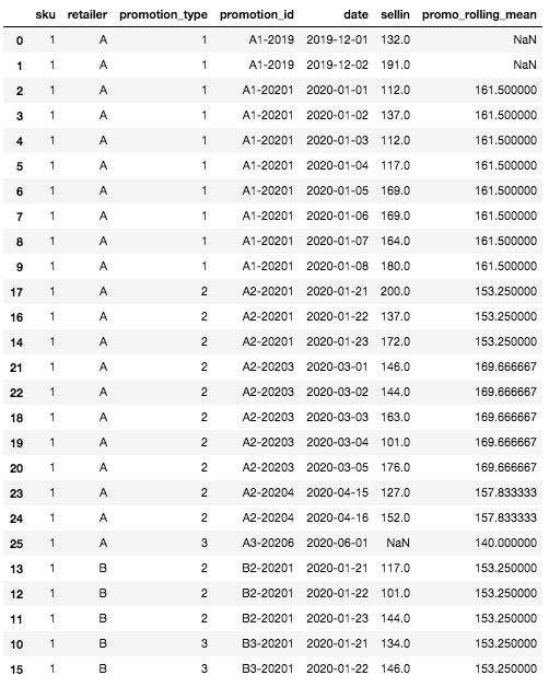
具有滚动平均值功能的最终 DataFrame
首先,我们可以看到 DataFrame 顶部的滚动平均值特征有一些缺失值。这是正常现象,因为对于第一行,我们没有任何 SKU 和零售商的历史记录,因此无法计算滚动平均值。这是滚动平均值为空的唯一情况,其他情况可以通过定义粒度聚合级别来处理。.
例如,对于我们在开头定义的特定行(SKU:1,零售商 A,促销类型:3,日期:2020-06-01),我们还不知道其卖出量,滚动平均值将是最相似和最近促销的卖出量平均值。因此,滚动平均值将是 SKU=1、促销类型=3、零售商=B 的销售额平均值,即:mean([134, 146]) = 140。.
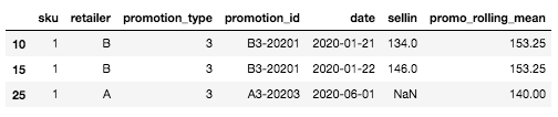
针对情侣 SKU x 零售商的新促销类型示例
这种逻辑可以扩展到这类项目中可能遇到的其他几种情况。例如,可以创建一个额外的层级,即产品系列,用于没有特定产品历史记录的情况。在这种情况下,我们将根据属于同一产品系列的产品取平均值。因此,重要的是要考虑这些粒度级别,并根据您自己对 “促销相似性 ”的定义来确定它们的优先级。.
您也可以衡量特定产品和特定客户的促销提升(即特定促销产生的额外销量),而不是滚动手段。这样做的目的是计算特定促销期间的销售额与未进行任何促销的销售额之间的比率。.
提示 4:处理大型 data
在这种粒度下工作会大大增加复杂性和对计算能力的需求。如果您和我们一样,需要处理数百个 SKU、零售商和数年的每日历史销售量,就必须找到并行计算的方法。例如,如果您不需要从其他 SKU 获取任何信息来实现促销功能,您可以在 sku 列上对 data 进行分区,然后使用分布式计算。我们发现使用 Dask 来完成这项任务非常有用:
从 dask 导入延迟、计算
def compute_rolling_mean(df):
...
返回 df
skus_list = set(df[‘sku’])
dfs_with_promo = [
delayed(compute_rolling_mean)(df.loc[df.sku == sku]) for skus_list 中的 sku
]
df_final = pd.concat(compute(*dfs_with_promo), axis=0, ignore_index=True)
提示 5:考虑到不同产品之间的需求转移
不要忘记,每个 SKU 的销售不仅会受到其促销活动的影响,还会受到可替代产品促销活动的影响,这种现象被称为 "蚕食"。为了建立一个性能良好的模型,必须预测 "蚕食 "可能会导致某些产品的销量下降。.
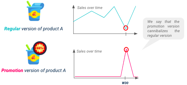
蚕食图解
为了能够对这一现象进行建模,我们首先必须检测产品之间的蚕食关系。主要有两种方法:
自动检测深潜
自动检测蚕食关系的一种方法是使用相关分数。这种方法不是根据产品类别,而是根据产品历史销售额变化之间的相关性,将真正有可能相互蚕食的产品集中在一起。我们会计算每对产品的相关性得分,如果相关性得分呈强负值,我们就可以认为这些产品会相互蚕食。
深度挖掘 "蚕食 "功能
根据这些蚕食关系,我们可以按照与直接促销相同的方法创建特征。例如
结果和结论
在我们的项目中,我们观察到,在大多数情况下,滚动平均值特征往往比上行/下行特征对模型更有效。例如,对于某个国家,滚动平均特征使预测精度提高了 2.8%,而上移特征则提高了 2%。.
然而,每个项目都不尽相同,我们的主要经验是,探索阶段至关重要,它是以后创建功能的基础。有必要真正了解促销活动的运作方式及其影响,以便为其建立正确的模型。这需要与业务所有者进行讨论,并进行探索性 Data 分析。.